大气散射 ( Atmosphere Scattering)
大气散射介绍
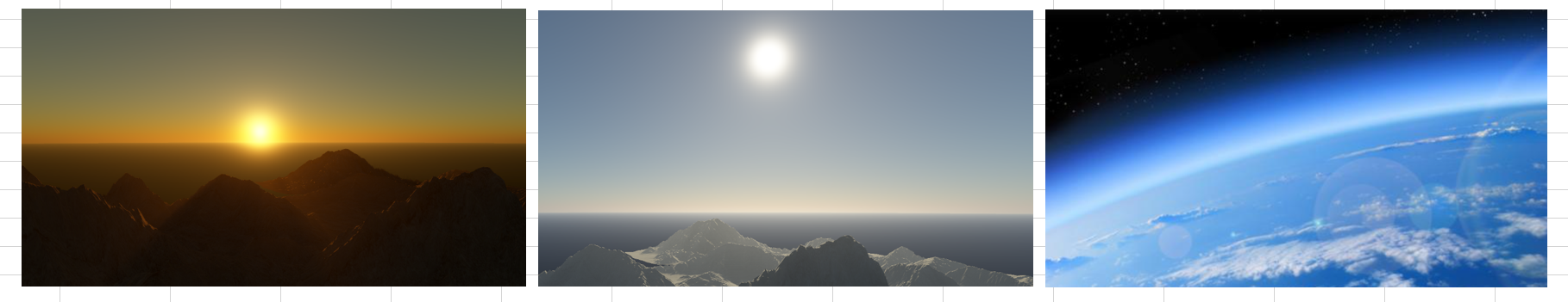
当你看到蓝天白云,日落黄昏,或者从太空遥望地球,地球周围一圈蓝色光晕,有没有想过这些现象产生的原因是什么?这些物理现象用一句话解释:太阳光与大气层中的参与介质发生了大气散射现象,从而形成了天空颜色
散射
光源的辐射沿着路径前行时,碰到参与介质时会发生几种不同散射现象的行为:
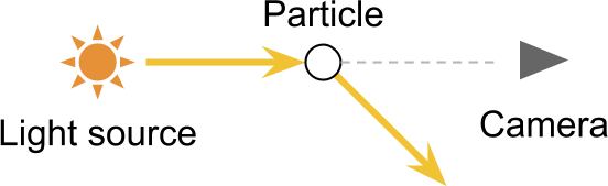
出射散射(Out-Scattering)
出射散射也就是光子碰到空气中的分子后,原本要射向摄像机的光线发生了偏转,光线的方向改变了![]()
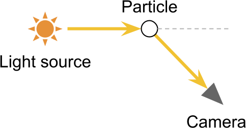
入射散射(In-Scattering)
入射散射与出射散射相反,本来不指向相机的光线也可能被偏转到相机的方向,这就是入射散射。![]()
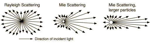
根据粒子大小不同可分为瑞利散射(Rayleigh Scattering) 和 米氏散射(Mie Scattering)
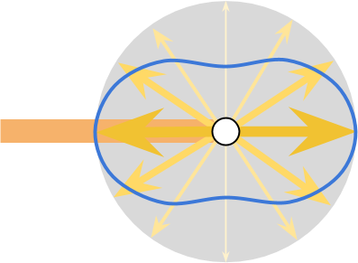
什么是散射?
光碰到不同大小粒子后发生散射,不同方向上的光强如下图,箭头长度表示光线强弱,箭头越长,光线越强。
大气散射模型
大气散射模型分为两种:Single Scattering和Multi Scattering。
Single Scattering 即只考虑太阳光经过一次散射后抵达我们的眼睛。
Multi Scattering,考虑光线多次散射过程的模型。显然这更符合现实世界的情况,但下一级的散射取决于与上一级散射的结果,也就是说这是一个递归方程,实现起来并不太容易。
模型简化
由于第二次散射以上的能量较少,对最终视觉的影响程度有限,所以目前Single Scattering 还是一种相对实现简单效果也不会差很多的模型,这里也主要介绍 Single Scattering。
因此单次散射大气模型求解问题如下:
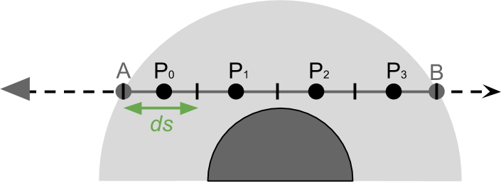
我们从路径 AB 观察大气,并且求解 B 点的大气颜色,光线在大气中只发生一次散射,散射点为 P:
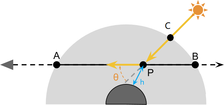
实际上在路径 AB 上有无数个 P 点,因此最终求解是对 AB 路径上每一个点的光照贡献进行累加(求积分)
因此整个模型可以分解成如下问题:
- P 点光照 :光线穿过大气会衰减,到达 P 点后的光照强度。
- 光线在 P 散射:进入相机方向的光照,即入射散射部分
- 累加所有 P 点光照
透射函数
为了计算散射点的光照,我们先考虑如下一段光线:
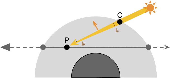
- 光线从太阳传到 C,此时是真空,所以没有损失,我们用 $I_C$ 指代 C 点的光强
- 在从 C 点到 P 点的过程在中,经过 CP 路径衰减,我们用 $I_P$ 指代 P 点的光强
- $I_P$ 比 $I_C$ 的值就是 透射率(Transimittance) :$T (CP) = \frac{I_P}{I_C}$
P 点的光强也就是:
$$I_P = I_C * \textcolor{Green}{T(CP)}$$
其中,T项是衰减系数(Transmittance),它表示在某段路径上的对光照的衰减程度。该公式也可以被认为是零级散射(zero scattering),即不考虑任何散射事件、直接考虑经过衰减后光强。
散射函数:S(λ,θ,h)
P点在接受光照后,会因为散射偏转一部分,于是我们需要散射函数 $S(\lambda,\theta,h)$ 来表示某一方向上光线的偏转情况。如下图,那些偏转了 $\theta$ 角的光线才能被指向A点的摄像机:
于是我们可以得出从 P 点出发到 A 点的光强:
$$I_{PA}=\boxed{I_P}\textcolor{Red}{S(\lambda,\theta,h)} \textcolor{Green}{T(PA)} $$
从公式中可以看出,散射跟角度 $\theta$、光线波长 $\lambda$ 以及 $P$ 点高度 $h$ 有关系。
散射类别
散射系数和粒子的大小和折射率有关,这里就得解释一下大气粒子的分类。我们知道大气中有很多不同种类的大气分子/粒子,一般在大气渲染模型里把它们分成两大类。一种是小分子,例如氮气和氧气分子等,另一种是大粒子,例如各种尘埃粒子。之所以要进行分类是因为它们对光线有着不一样的行为(这里忽略对光的吸收,只考虑散射):
- 小分子:指大小远小于光线波长的粒子。小分子对光的散射在前后方向上分布比较均匀,通常会使用 Rayleigh散射(Rayleigh Scattering) 对它们进行建模。由于这些分子大小比波长还要小很多,因此光的波长也会影响 Rayleigh 散射的程度。
- 大粒子:指大小远大于光线波长的粒子。大粒子在发生散射的时候会把更多的光散射到前向,通常会使用 Mie散射(Mie Scattering) 对它们进行建模。由于光的波长相较于这些粒子大小来说是可以忽略的,因此我们认为 Mie 散射跟光线波长无关。
Rayleigh 散射
对于足够小的粒子,光线在撞击它后会经历什么?我们通常使用瑞利散射来建模。
Rayleigh 散射曲线图如下:

散射函数如下,这个方程并不是真正的Rayleigh散射方程,你去维基百科里面查,会发现另外一个公式,这个公式来自这篇论文:
$$\textcolor{Red}{S(\lambda,\theta,h)} = \frac{\pi2(n2-1)2}{2}\frac{\textcolor{Gold}{\rho(h)}}{N}\frac{1}{\lambda4}(1+cos\theta^2)$$
其中,
- $\lambda$ 是光的波长
- $n=1.00029$ 是粒子折射率
- $N=2.504*10^{25}$ 是海平面处的大气密度,单位是 分子数/立方米
- $\rho(h)$ 是高度 $h$ 处的相对大气密度(即相对于海平面的密度,可以理解成 $h$ 处真正的大气密度与海平面处大气密度的比值,因此它在海平面处值为 1,随着 $h$ 增加不断减小),我们一般会使用指数函数对它的真实曲线进行数学拟合(是一种近似拟合,不要和后面提到的指数函数弄混):
$$\textcolor{Gold}{\rho(h)}=exp(-\frac{h}{H})$$
其中 H 为 “Scale Height”,相当于是一个基准的高度。
- 对于 Rayleigh 来说,H= 8500米。
- 对于 Mie 来说,H = 1200米。
可以看出Rayleigh散射大致和波长的4次幂的成反比,波长越小(越靠近紫光)的光被散射得越厉害。所以白天的时候天空为蓝色,因为蓝光在大气里不断被散射,黄昏的时候天空会变红,因为相比于白天,阳光此时要穿越更厚得多的大气层,在到达人眼之前,大多数蓝光都被散射到其他方向,所以剩下来的就是红光了。

Rayleigh 散射系数
Rayleigh 散射的公式 $S(\lambda,\theta,h)$ 表示在某个特定方向上的光强度,要求总散射系数就需要对散射函数做球面积分:
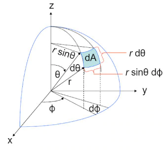
Tips
球面积分示意图,这里假定 r 等于 1,对球面积分时,因为 $d\theta$ 跟 $d\phi$ 非常小,因此球面可以看成是矩形,因此蓝色框长度为 $w=rsin\theta d\phi$ (弦长公式:蓝色面片上边缘半径 $rsin\theta$,角度 $d\phi$),高为 $d\theta$,则面积 $S=rsin\theta d\phi d\theta$
因此:
$$\beta(\lambda, h) = \int_{0}{2\pi}{\int_{0}{\pi}{S(\lambda,\theta,h)}sin\theta d\theta d\phi}$$
最后得出:
$$\beta(\lambda, h) = \frac{8\pi3(n2-1)2}{3}\frac{\textcolor{Gold}{\rho(h)}}{N}\frac{1}{\lambda4}$$
特别地,当 $h=0$ 时,即表示海平面的散射系数:
$$ \beta(\lambda, 0) = \frac{8\pi3(n2-1)^2}{3} \frac{ \textcolor{Gold}{1} }{N} \frac{1}{\lambda^4} $$
举例来说就,对于红绿蓝的波长,在海平面时,可以得出这些结果:
$$\begin{aligned}
\beta(\textcolor{Red}{680nm}) &= 5.210^{-6} \
\beta(\textcolor{Green}{550nm}) &= 12.110^{-6} \
\beta(\textcolor{DodgerBlue}{440nm}) &= 29.6*10^{-6}
\end{aligned}$$
有些技术帖跟论文里计算结果如下: $\beta_rrgb=(5.8, 13.5, 33.1) \cdot 10{-6}$,$n=1.0003,N=2.545\cdot10{25}$
>>> 8*math.pi**3*(1.00029**2-1)**2/3.0/(2.504e25)/((680e-9)**4)
5.196731735928312e-06
>>> 8*math.pi**3*(1.00029**2-1)**2/3.0/(2.504e25)/((550e-9)**4)
1.2142697926864656e-05
>>> 8*math.pi**3*(1.00029**2-1)**2/3.0/(2.504e25)/((440e-9)**4)
2.964525861050941e-05
总散射系数公式也可以拆解为:
$$\beta(\lambda, h) = \frac{8\pi3(n2-1)2}{3}\frac{\textcolor{Gold}{\rho(h)}}{N}\frac{1}{\lambda4}=\beta(\lambda) \textcolor{Gold}{\rho(h)}$$
其中:
$$\beta(\lambda) = \frac{8\pi3(n2-1)2}{3}\frac{1}{N}\frac{1}{\lambda4}$$
Rayleigh 相位函数
Rayleigh 散射的原方程可以分解成两个分量,一个是上面的有关能量强度的散射系数,另一个分量则和它几何形状有关
$$S(\lambda,\theta,h)=\beta(\lambda, h)\underbrace{\gamma(\theta)}_{geometry}$$
$\gamma(\theta)$ 可以用前两者之比得到。
$$\begin{aligned}
\gamma(\theta) &= \frac{S(\lambda,\theta,h)}{\beta(\lambda, h)}\
&=\frac{3}{16\pi}(1+cos^2\theta)
\end{aligned}$$
该表达式不依赖波长,$\gamma(\theta)$ 的函数图像就是之前两瓣的偶极子形状
PS: 整个散射函数可以拆分成 $\textcolor{Red}{S(\lambda,\theta,h)}= \textcolor{DodgerBlue}{ \beta(\lambda)} \textcolor{Gold}{\rho(h)} \textcolor{Purple}{\gamma(\theta)}$
Mie 散射
光线的散射是很复杂的,瑞利散射对原子和分子可以有效模拟,但是对光线和大物体(气溶胶)的交互没什么作用。地球大气布满了气溶胶,所以仅是瑞利散射是不足以复现的,为此常用的就是 米氏散射(Mie scattering),这种散射类型倾向于扩散光线,让光源看起来比实际大,但不会改变光的颜色
Mie 散射系数
米散射系数很难去推导计算,基于统计数据的结果,米散射系数可以常量进行估计。论文10中给出海平面的米散射系数:
$$\beta(\textcolor{Red}{680nm},\textcolor{Green}{550nm} ,
\textcolor{DodgerBlue}{440nm} = (2.210^{-5}, 2.210^{-5}, 2.2*10^{-5})$$
Mie 散射相位函数
真实的 Mie 散射相位函数图像如下:
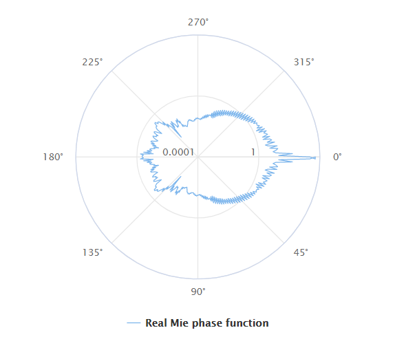
因此 Mie 相位函数也是近似方式得出,我们可以利用Henyey-Greenstein 函数,该函数在1941年提出:
$$\gamma_{HG}(\theta)=\frac{1}{4\pi}\frac{1-g2}{(1+g2-2gcos\theta)^\frac{3}{2}}$$
在 1992 年 Cornette 对其进行了改进:
$$\gamma_{M}(\theta)=\frac{3}{8\pi}\frac{1-g2}{(2+g2)}\frac{1+cos2\theta}{(1+g2-2gcos\theta)^\frac{3}{2}}$$
该函数引入了一个参数 $g(-1<g<1)$,决定了前后散射的相对强度,代表散射方向的平均余弦。正的 $g$ 值会增加正向散射的光量,负的 $g$ 值表示向后散射的光量。 $g=0$ 的值导致各向同性散射。
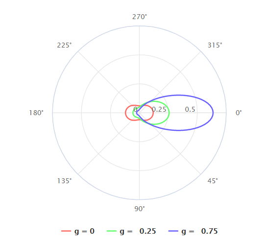
对于地球大气层,一般可以取 $g=0.758$。然后由于上述两个函数计算成本比较高,快速应用可以使用 Schlick 相位函数:
$$\lambda_S(\theta)=\frac{1}{4\pi}\frac{1-g2}{(1+gcos\theta)2}$$
衰减系数 $\textcolor{Green}{T}$
$T(a,b)$ 表示 $a,b$ 之间的透射率(transmittance),其定义为9:
$$T(a,b)=exp(-\int_a^b\sigma_t(p)dl_p$$
其中 $\sigma_t$ 为介质衰减系数,
Rayleigh
在大气中,Rayleigh 散射可以用 Rayleigh theory 近似描述:$\sigma_RT(h,\lambda)=\beta(\lambda, h)$
即:
$$\textcolor{Green}{T(PA)}=exp{-\int_P^A{\textcolor{DodgerBlue}{\beta(\lambda, h)}}ds}$$
带入之前求解的总散射系数公式: $\beta(\lambda,h)$
$$\textcolor{Green}{T(PA)}=exp{-\textcolor{DodgerBlue}{\beta(\lambda)}\int_P^A{\textcolor{Gold}{\rho(h)}}ds}$$
其中的积分项对应的是路径长度 $x$,可以理解为在光传播路径上,对大气密度函数 $\textcolor{Gold}{\rho(h)}$ 求积分,这部分被称为 光学距离——Optical Depth:
$$\textcolor{Darkorange}{D(PA)}=\int_P^A{\textcolor{Gold}{\rho(h)}}ds}$$
总结
至此,我们简单推导了 $S$ 跟 $T$,这样一开始的公式可以写成:
$$\begin{aligned}
I_{PA} &= \boxed{I_P}\textcolor{Red}{S(\lambda,\theta,h)} \underline {\textcolor{Green}{T(PA)} } \
&=\boxed{I_S\textcolor{Green}{T(CP)}} \textcolor{Red}{S(\lambda,\theta,h)} \underline { \textcolor{Green}{T(PA)} } \
&= \boxed { I_S {exp{-\textcolor{DodgerBlue}{\beta(\lambda)}\textcolor{Darkorange}{D(CP)}}} } \textcolor{Red}{ { \textcolor{DodgerBlue}{ \beta(\lambda)} \textcolor{Gold}{\rho(h)} \textcolor{Purple}{\gamma(\theta)} } } \underline { {exp{-\textcolor{DodgerBlue}{\beta(\lambda)}\textcolor{Darkorange}{D(PA)}}} }\
&= I_S \textcolor{Red}{ { \textcolor{DodgerBlue}{\beta(\lambda)} \textcolor{Gold}{\rho(h)} \textcolor{Purple}{\gamma(\theta)} } } {exp{ -\textcolor{DodgerBlue}{\beta(\lambda)} { \textcolor{Darkorange}{D(CP)} + \textcolor{Darkorange}{D(PA)} } } }
\end{aligned} $$
其中,一般情况下,太阳光照角度固定,可以看成是平行光,$\textcolor{Purple}{\gamma(\theta)}$ 可以看成常量,$\textcolor{DodgerBlue}{\beta(\lambda)}$ 也是常量,也就是海平面附近的散射系数,在 Shader 中作为输入即可,$\textcolor{Darkorange}{D(PA)}$ 等在 Shader 中计算。
总结起来,公式表示的含义就是,计算观察路径AB上某一点P的光照贡献:
- 光线从太阳出发,到达大气边缘的C点
- 经过路径CP上的衰减到达P点(0级散射)
- 在P点发生一次散射,将一部分光散射到了观察方向上(1级散射)
- 这部分光又经过AP路径上的衰减最终到达了我们的眼睛
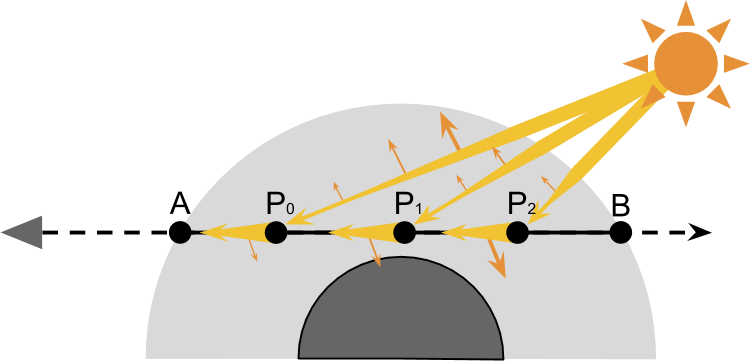
数值积分
P只是AB上的某一点,我们需要对路径AB上的每一点进行积分:
$$\begin{aligned}
I_A &= \sum_{i=0}^{n}I_{P_n} \
&= \int_{A}^{B} I_{PA} ds \
&= \int_{A}^{B} I_S \textcolor{Red}{ { \textcolor{DodgerBlue}{\beta(\lambda)} \textcolor{Gold}{\rho(h)} \textcolor{Purple}{\gamma(\theta)} } } { exp{ -\textcolor{DodgerBlue}{\beta(\lambda)} { \textcolor{Darkorange}{D(CP)} + \textcolor{Darkorange}{D(PA)} } } } ds \
&= I_S \textcolor{DodgerBlue}{\beta(\lambda)} \textcolor{Purple}{\gamma(\theta)} \int_{A}^{B} {exp{ -\textcolor{DodgerBlue}{\beta(\lambda)} { \textcolor{Darkorange}{D(CP)} + \textcolor{Darkorange}{D(PA)} } }} \textcolor{Gold}{\rho(h)} ds
\end{aligned} $$
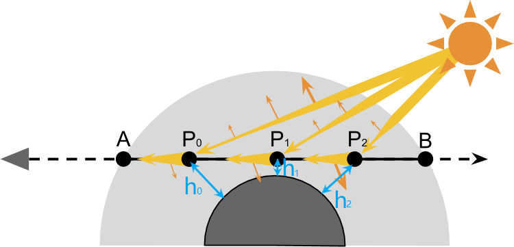
Tips
在大气shader中,我们将 $AB$ 分割成等长的若干段,然后取这些段的中点记为 $P_i$,然后分别计算每个点的 $I_{P_i}$,最后将这些点的光照累加起来。
大气球体shader框架思路
光线与大气相交
从之前得出的公式中可以得知,我们需要在 $AB$ 路径上求光学距离,我们第一步需要求出 $AB$ 的长度:
如下图所示,灰色部分是大气,我们需要求出观察路径 $AB$,其中已知:
- $O$:相机位置
- $C$:大气球心位置
- $L$:相机到大气球心长度
- $R$:大气球半径
- $\vec{OD}$ :观察方向,单位向量
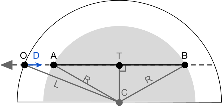
如图可以依次求出,
- $OT = \vec{OC} \cdot \vec{OD}$
- $TC = \sqrt{L^2 - OC^2}$
- $AT = \sqrt{R^2 - TC^2}$
- $OA = OT-AT$
- $OB = OT+BT=OT+AT$
bool RayIntersect(
    // Ray
    float3 O, // Origin
    float3 D, // Direction

    // Sphere
    float3 C, // Centre
    float R,    // Radius
    out float AO, // First intersection time
    out float BO  // Second intersection time
)
{
    float3 L = C - O;
    float DT = dot (L, D);
    float R2 = R * R;

    float CT2 = dot(L,L) - DT*DT;

    // CT 长度超过了求半径 R,此时视线跟大气不相交
    // Intersection point outside the circle
    if (CT2 > R2)
        return false;

    float AT = sqrt(R2 - CT2);
    float BT = AT;

    AO = DT - AT;
    BO = DT + BT;
    return true;
}
光线与行星相交
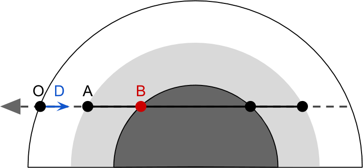
视线有可能会被行星阻挡,因此需要做两次相交函数,一次判断大气,一次判断行星。
// Intersections with the atmospheric sphere
//     D    : 观察方向向量
// worldPos : 相机坐标
float tA;    // Atmosphere entry point (worldPos + D * tA)
float tB;    // Atmosphere exit point  (worldPos + D * tB)
if (!RayIntersect(O, D, _PlanetCentre, _AtmosphereRadius, tA, tB))
    return fixed4(0,0,0,0); // The view rays is looking into deep space

// Is the ray passing through the planet core?
float pA, pB;
if (RayIntersect(O, D, _PlanetCentre, _PlanetRadius, pA, pB))
    tB = pA;
采样视线
之前我们得到了 $AB$ 路径上每个点 $P$ 的光照公式:
$$\begin{aligned}
I_A &= I_S \textcolor{DodgerBlue}{\beta(\lambda)} \textcolor{Purple}{\gamma(\theta)} \int_{A}^{B} {exp{ -\textcolor{DodgerBlue}{\beta(\lambda)} { \textcolor{Darkorange}{D(CP)} + \textcolor{Darkorange}{D(PA)} } }} \textcolor{Gold}{\rho(h)} ds \
&= I_S \textcolor{DodgerBlue}{\beta(\lambda)} \textcolor{Purple}{\gamma(\theta)} \sum_{P \in AB} \textcolor{Green}{T(CP)} \textcolor{Green}{T(PA)} \textcolor{Gold}{\rho(h)} ds
\end{aligned}$$
线段上有无数个 $P$ 点,为了近似求解 $I$,我们需要把线段划分为数个长度为 $ds$ 的小段
$AB$ 被划分的段数,就是视线采样数(View Samples),在 Shader 可以这么处理:
// Numerical integration to calculate
// the light contribution of each point P in AB
float3 totalViewSamples = 0;
float time = tA;
float ds = (tB - tA) / (float)(_ViewSamples);
for (int i = 0; i < _ViewSamples; i ++)
{
    // Point position
    // (sampling in the middle of the view sample segment)
    // O : 相机位置
    // D : 相机方向向量
    float3 P = O + D * (time + ds * 0.5);

    // T(CP) * T(PA) * ρ(h) * ds
    totalViewSamples += ViewSampling(P, ds);

    time += ds;
}

// I = I_S * β(λ) * γ(θ) * totalViewSamples
float3 I = _SunIntensity *  _ScatteringCoefficient * phase * totalViewSamples;
接下来就是求解每个 $P$ 点上的 $\textcolor{Green}{T(CP)} \textcolor{Green}{T(PA)} \textcolor{Gold}{\rho(h)}ds$
光学深度 $PA$
回顾一下之前的公式:
$$ \textcolor{Green}{T(CP)} \textcolor{Green}{T(PA)} = exp{ -\textcolor{DodgerBlue}{\beta(\lambda)} { \textcolor{Darkorange}{D(CP)} + \textcolor{Darkorange}{D(PA)} } }$$
其中:
$$\textcolor{Darkorange}{D(PA)}=\sum_{Q \in PA} exp { -\frac{h_Q}{H} }ds$$
$h_Q$ 表示当前点的高度,有一点注意 $\textcolor{Gold}{\rho(h)}=exp(-\frac{h_Q}{H})$,这里顺便可以求解 $AB$ 上的积分 $\textcolor{Gold}{\rho(h)}ds$。
Shader 实现如下:
// + Accumulator for the optical depth
float opticalDepthPA = 0;

float3 totalViewSamples = 0;
float time = tA;
float ds = (tB - tA) / (float)(_ViewSamples);
for (int i = 0; i < _ViewSamples; i ++)
{
    float3 P = O + D * (time + ds * 0.5);

    ///////// Begin ViewSampling()
    // T(CP) * T(PA) * ρ(h) * ds

    // 1: ρ(h) * ds

    //            C : 行星球形坐标
    // _ScaleHeight : Rayleigh/Mie 散射里的基准高度

    float height = distance(C, P) - _PlanetRadius;
    float opticalDepthSegment = exp(-height / _ScaleHeight) * ds;


    // 2: D(PA)
    opticalDepthPA += opticalDepthSegment;

    ////////    End ViewSampling()

    time += ds;
}

// I = I_S * β(λ) * γ(θ) * totalViewSamples
float3 I = _SunIntensity *  _ScatteringCoefficient * phase * totalViewSamples;
光学深度 $CP$
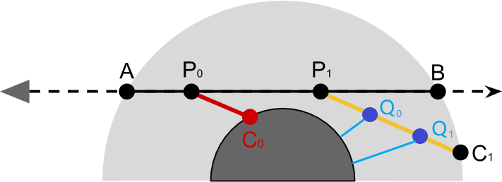
累加符号里 $P$ 点的光量贡献还剩下 $CP$ 的光学深度,我们在求 $CP$ 的光学深度时,建立一个 LightSampling 方法,也就从 $P$ 点出发指向太阳进行采样,把太阳的出射点叫做 $C$ (注意跟之前的球心坐标 $C$ 区分),然后注意下面 $C_0$ 的情况,光线被星球遮挡,此时要忽略 $P_0$ 点的贡献。
Shader 实现如下:
bool LightSampling(
    float3 P,    // Current point within the atmospheric sphere
    float3 S,    // S 是光照方向,从 P 点到 C 点的平行光
    out float opticalDepthCA
)
{
    float _; // don't care about this one

    // 这里 C 是局部变量,表示光线在大气表面的入射点
    float C;
    RayInstersect(P, S, _PlanetCentre, _AtmosphereRadius, _, C);

    // Samples on the segment PC
    // _LightSamples : CP 上的分段次数

    float time = 0;
    float ds = distance(P, P + S * C) / (float)(_LightSamples);
    for (int i = 0; i < _LightSamples; i ++)
    {
        // Q 点如上图所示
        // S : 光照方向
        float3 Q = P + S * (time + lightSampleSize * 0.5);
        float height = distance(_PlanetCentre, Q) - _PlanetRadius;
        // Inside the planet
        if (height < 0)
            return false;

        // Optical depth for the light ray
        opticalDepthCA += exp(-height / _RayScaleHeight) * ds;

        time += ds;
    }

    return true;
}
然后之前的代码加入 $CP$ 的计算如下:
float opticalDepthPA = 0;

float3 totalViewSamples = 0;
float time = tA;
float ds = (tB - tA) / (float)(_ViewSamples);
for (int i = 0; i < _ViewSamples; i ++)
{
    float3 P = O + D * (time + ds * 0.5);

    ///////// Begin ViewSampling()
    // T(CP) * T(PA) * ρ(h) * ds

    // ρ(h) * ds
    float height = distance(C, P) - _PlanetRadius;
    float opticalDepthSegment = exp(-height / _ScaleHeight) * ds;

    // D(PA)
    opticalDepthPA += opticalDepthSegment;

    // D(CP)
    float opticalDepthCP = 0;
    bool overground = LightSampling(P, S, opticalDepthCP);

    if (overground)
    {
        // Combined transmittance
        // T(CP) * T(PA) = T(CPA) = exp{ -β(λ) [D(CP) + D(PA)]}
        float3 transmittance = exp(
            -_ScatteringCoefficient *
            (opticalDepthCP + opticalDepthPA)
        );

        // Light contribution
        // T(CPA) * ρ(h) * ds
        totalViewSamples += transmittance * opticalDepthSegment;
    }

    ////////    End ViewSampling()

    time += ds;
}

// I = I_S * β(λ) * γ(θ) * totalViewSamples
float3 I = _SunIntensity *  _ScatteringCoefficient * phase * totalViewSamples;
散射系数
之前我们重点以 Rayleigh 散射来介绍如何计算单次大气散射,接下来加上 Mie 散射,之前的方程:
$$\begin{aligned}
I &= I_S \textcolor{DodgerBlue}{\beta(\lambda)} \textcolor{Purple}{\gamma(\theta)} \sum_{P \in AB} L(P) \
\end{aligned}$$
加上 Mie 反射后:
$$\begin{aligned}
I &= \overbrace{ I_S \textcolor{DodgerBlue}{\beta_R(\lambda)} \textcolor{Purple}{\gamma_R(\theta)} \sum_{P \in AB} L_R(P) }^{Rayleigh \ Scattering} + \overbrace{ I_S \textcolor{DodgerBlue}{\beta_M(\lambda)} \textcolor{Purple}{\gamma_M(\theta)} \sum_{P \in AB} L_M(P) }^{Mie \ Scattering} \
&=I_S \left( \overbrace{ \textcolor{DodgerBlue}{\beta_R(\lambda)} \textcolor{Purple}{\gamma_R(\theta)} \sum_{P \in AB} L_R(P) }^{Rayleigh \ Scattering} + \overbrace{ \textcolor{DodgerBlue}{\beta_M(\lambda)} \textcolor{Purple}{\gamma_M(\theta)} \sum_{P \in AB} L_M(P) }^{Mie \ Scattering} \right)
\end{aligned}$$
因此代码实现也需要做修改:
bool LightSampling(
    float3 P,
    float3 S,
    // Modify : float ->  float2
    // 分别计算光学深度 .xy  ->  Rayleight Mie
    out float2 opticalDepthCA
)
{
    float _;
    float C;
    RayInstersect(P, S, _PlanetCentre, _AtmosphereRadius, _, C);

    float time = 0;
    float ds = distance(P, P + S * C) / (float)(_LightSamples);
    for (int i = 0; i < _LightSamples; i ++)
    {
        float3 Q = P + S * (time + lightSampleSize * 0.5);
        float height = distance(_PlanetCentre, Q) - _PlanetRadius;
        if (height < 0)
            return false;

        // 分别计算 Rayleigh、Mie 的光学深度,基准的高度值不一样
        opticalDepthCA.x += exp(-height / _RayScaleHeight.x) * ds;
        opticalDepthCA.y += exp(-height / _RayScaleHeight.y) * ds;

        time += ds;
    }

    return true;
}
// Modify : float -> float2
float2 opticalDepthPA = 0;
float3 totalRayViewSamples = 0;
float3 totalMieViewSamples = 0;
float time = tA;
float ds = (tB - tA) / (float)(_ViewSamples);
for (int i = 0; i < _ViewSamples; i ++)
{
float3 P = O + D * (time + ds * 0.5);
///////// Begin ViewSampling()
// T(CP) * T(PA) * ρ(h) * ds
// ρ(h) * ds
float height = distance(C, P) - _PlanetRadius;
// float -> float2
float2 opticalDepthSegment = 0;
opticalDepthSegment.x = exp(-height / _ScaleHeight.x) * ds;
opticalDepthSegment.y = exp(-height / _ScaleHeight.y) * ds;
// D(PA)
opticalDepthPA += opticalDepthSegment;
// D(CP)
// Modify : float -> float2
float2 opticalDepthCP = 0;
bool overground = LightSampling(P, S, opticalDepthCP);
if (overground)
{
// Combined transmittance
// T(CP) * T(PA) = T(CPA) = exp{ -β(λ) [D(CP) + D(PA)]}
float3 transmittanceRay = exp(
-_RayScatteringCoefficient *
(opticalDepthCP.x + opticalDepthPA.x)
);
float3 transmittranceMie = exp(
-_MieScatteringCoefficient *
(opticalDepthCP.x + opticalDepthPA.y)
);
// Light contribution
// T(CPA) * ρ(h) * ds
totalRayViewSamples += transmittanceRay * opticalDepthSegment;
totalMieViewSamples += transmittanceMie * opticalDepthSegment;
}
//////// End ViewSampling()
time += ds;
}
// I = I_S [βr(λ) * γr(θ) * totalRayViewSamples
// + βm(λ) * γm(θ) * totalMieViewSamples)
float3 I = _SunIntensity * (
_RayScatteringCoefficient * rayPhase * totalRayViewSamples +
_MieScatteringCoefficient * miePhase * totalMieViewSamples
);其中常量部分:
$_RayScatteringCoefficient(\textcolor{Red}{680nm},\textcolor{Green}{550nm},\textcolor{DodgerBlue}{440nm}) = (5.8, 13.5, 33.1)*10^{-6}$
$_MieScatteringCoefficient(\textcolor{Red}{680nm},\textcolor{Green}{550nm},\textcolor{DodgerBlue}{440nm})=(2.2, 2.2, 2.2)*10^{-5}$
$rayPhase$、$miePhase$ 提前计算好的相位函数值,如果光源会改变方向,可以在 Shader 中增加函数来计算数值。
$_ScaleHeight=(8500, 1200)$
参考资料
1.Volumetric Atmospheric Scattering
5.Extended Disney “principled” Shader